Let’s face it – time series forecasting can be a bit of a puzzle.
One minute you’re dealing with trends, the next you’re battling seasonality.
And let’s not even get started on those pesky external factors that seem to pop up out of nowhere. It’s enough to make your head spin!
The biggest challenge? Creating a model that can keep up with the ever-changing dynamics of your data.
But fear not, there’s a solution!
Say hello to the Walk Forward Method, your new best friend in the world of time series forecasting.
What’s the Walk Forward Method, you ask?

Think of it as a way to keep your model on its toes.
Instead of training it once and calling it a day, the Walk Forward Method continuously retrains your model as new data rolls in.
It’s like having a personal trainer for your forecasting model, ensuring it’s always in tip-top shape and ready to tackle whatever challenges come its way.
Key Concepts
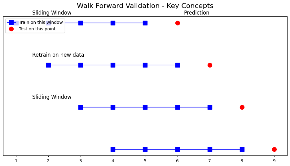
- Sliding Window: Imagine a window that moves along your data, training the model on a fixed chunk of past data and then testing it on the next data point.
- Dynamic Retraining: After each prediction, the window slides forward, incorporating the new data, and the model gets a quick refresher course.
- Sequential Forecasting: It’s all about taking things one step at a time. The model predicts the next time step, and then that prediction becomes part of the training data for the next round.
Why Bother with the Walk Forward Method?
In the real world, time series data is rarely static.
Market conditions change, seasons come and go, and unexpected events can throw a wrench in the works.
A model trained on old data might become as outdated as last year’s fashion trends.
That’s where the Walk Forward Method steps in:
- Continuous Adaptation: Your model evolves with the data, becoming more resilient to changes in trends and patterns.
- Better Accuracy: By training on the latest and greatest data, your model stays sharp and delivers more accurate forecasts.
- No More Overfitting: Training on different subsets of data helps prevent overfitting, a common problem where your model becomes too attached to one specific dataset and struggles to generalize to new data.
How Does it Actually Work?
Let’s break it down into simple steps:
- Train on Initial Window: Start by training your model on a chunk of your data (say, the first 80%).
- Make a Forecast: Use your trained model to predict the next data point.
- Update the Window: Slide that training window forward, including the latest actual data point.
- Repeat: Keep going, repeating steps 2 and 3 until you’ve covered all your data.
Let’s paint a picture…
Imagine you have data on monthly sales for the past five years. You want to predict sales for the next few months. Here’s what you could do:
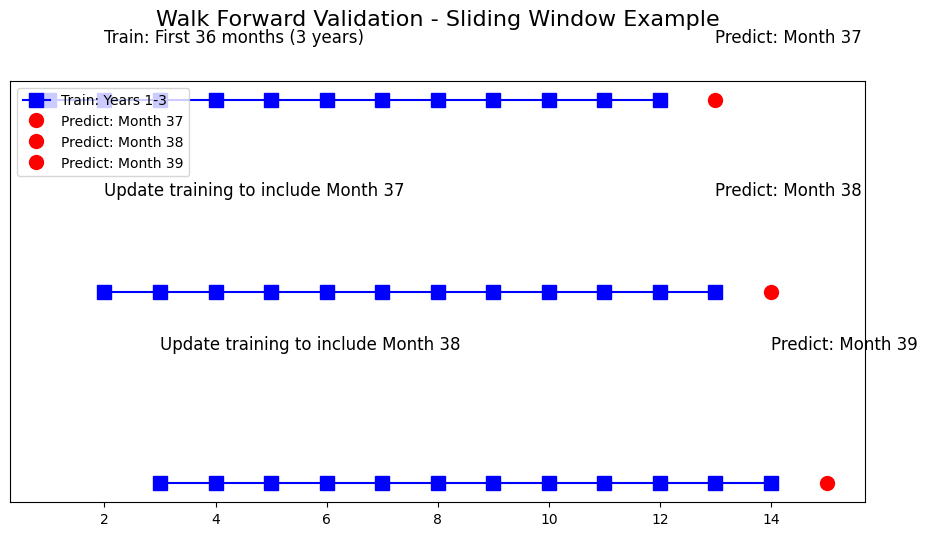
- Train your model on the first three years of data.
- Predict sales for month 37.
- Update your training data to include month 37 and predict month 38, and so on.
With each prediction, your model gets a little smarter.

Python Code Example – Let’s Get Practical!
import numpy as np
import pandas as pd
from statsmodels.tsa.arima.model import ARIMA
from sklearn.metrics import mean_squared_error

# Assuming 'sales_series' contains the data
np.random.seed(0)
time = np.arange(1, 101)
sales = 50 + 2 * time + np.random.normal(0, 10, len(time))  # Trend with noise
sales_series = pd.Series(sales)

# Split into train and test sets
train_size = int(len(sales_series) * 0.8)  # First 80% for training
train, test = sales_series[:train_size], sales_series[train_size:]

# Convert train and test to lists for easy appending and indexing
history = list(train)  # Initial training set
test_list = list(test)  # Convert test to a list
predictions = []

# Walk Forward Validation
for t in range(len(test_list)):
    # Train ARIMA model on current history
    model = ARIMA(history, order=(5, 1, 0))  # Example ARIMA(5,1,0)
    model_fit = model.fit()

    # Make forecast for the next step
    forecast = model_fit.forecast(steps=1)
    predictions.append(forecast[0])

    # Add the actual observation from the test set to the history
    history.append(test_list[t])

# Evaluate forecast performance using RMSE
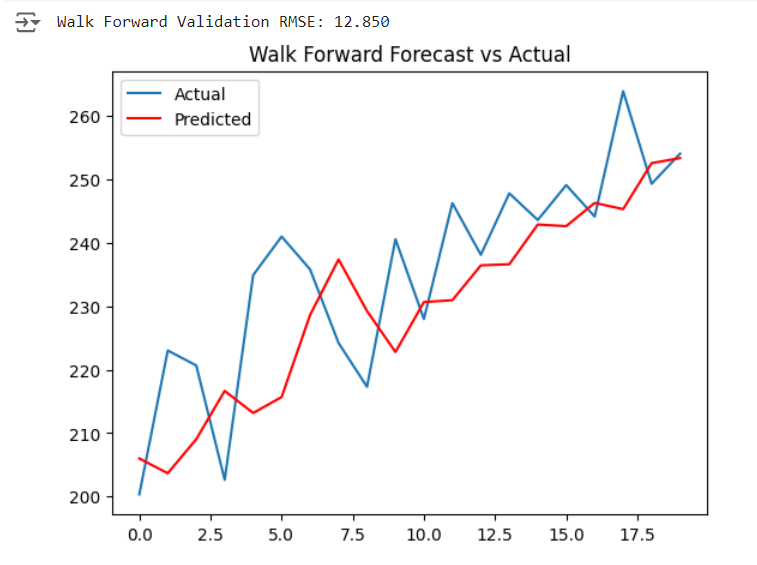
rmse = np.sqrt(mean_squared_error(test_list, predictions))
print(f'Walk Forward Validation RMSE: {rmse:.3f}')

# Plot results
import matplotlib.pyplot as plt
plt.plot(test_list, label='Actual')
plt.plot(predictions, label='Predicted', color='red')
plt.legend()
plt.title('Walk Forward Forecast vs Actual')
plt.show()
Code Walkthrough:
- Data Generation: We create a simple time series with a trend and some random noise to mimic real-world data.
- Train/Test Split: The first 80% is for training, the rest for testing.
- Walk Forward Validation: We train an ARIMA model, make a forecast, and then update the training data.
- Evaluation: We calculate the Root Mean Squared Error (RMSE) to see how well our model did and plot the results.
Output:

Advantages of the Walk Forward Method
- Realistic Testing: It’s like a dress rehearsal for your model, closely simulating how forecasts are made in the real world.
- No Data Leakage: By constantly updating the training data and testing on unseen data, we avoid any sneaky data leakage.
- Adaptive Modeling: Your model learns and adapts as new data comes in, ensuring it stays relevant.
Limitations – Let’s Keep it Real
- Computationally Intensive: Retraining the model for each forecast can take some time, especially with large datasets or complex models.
- Sensitive to Noise: If your data is noisy, the model might overreact to short-term fluctuations.
When to Use the Walk Forward Method
- Non-Stationary Data: If your data has changing trends or seasonality, this method is your go-to.
- Dynamic Environments: Think finance, retail, or weather forecasting – anywhere where recent data is key for future predictions.
- Continuous Learning: When your model needs to keep learning and updating, the Walk Forward Method is ideal.
Wrapping Up
The Walk Forward Method is a powerful tool for evaluating and improving time series models in dynamic environments.
It’s like giving your model a continuous learning experience, ensuring it stays sharp and delivers the best possible forecasts.
Now it’s Your Turn!
Give the Walk Forward Method a try on your own time series data.
Experiment with different models and see how it compares to traditional methods.
Remember, the world of time series forecasting is constantly evolving, and the Walk Forward Method is a great way to stay ahead of the curve.
Happy Forecasting!
Additional Resources:
P.S. If you have any questions or want to dive deeper into the world of time series forecasting, leave a comment below!
